This week I mostly finished Artillery, the simple game I am working on. I created a new projectile type (a homing projectile) and created some new levels, in addition to fixing some bugs and doing some texturing. I started the project principally to force myself to improve my knowledge of vectors, 3D Mathematics, and physics which I certainly did do. I am not sure if I will upload the finished game, the graphics are quite basic, and the multiplayer functionality is untested, I don’t know if it’s quite ready for upload. I may release it as “beta” software.
I build a simple 300 mW Infrared laser illuminator as well. It’s nothing complicated, I just wanted to boost the effectiveness of the Generation 1 night vision equipment that I have, and this is an excellent way of doing it. I found that in order to produce a properly collimated and circularised beam I need to do some “Beam forming” or “Beam shaping” using various different kinds of optics, mostly involving cylinder lenses.
I did a writeup of the Emergent AI project that I created the concept test for, and decided to postpone it. It is an exciting area of research, but I just feel that there is not enough material in the idea that I had to justify devoting an entire project to. I would basically be creating a system that searches for the optimum set of variables to solve a given problem, and while this would be interesting, I want to wait until I have fleshed out the idea more before I spend time on it.
I have come up with several excellent ideas for the new year, which I am very excited about. I have started research on them already, and even started development on one, but I won’t mention them until I officially start the projects in a few days.
This week I finished the Fast Fourier Transform and data recorder program (Project 115). There are a few improvements and GUI additions I would need to make before I would consider releasing it, but it does what I designed it to do.
I also bought the parts for an IR laser illuminator, in the 300mW range. I own a basic night vision monocular, and having an IR laser illuminator greatly boosts it’s range. I built a small low-power laser some time ago, and it worked well, so I thought I would build a more powerful model.
I finally released my Fluid Dynamics resource on GarageGames, which I talked about here.
With regards to the Resonat Inductive Coupler project, the concept I have is working, but is nowhere near powerful enough to move ahead in the project yet. I will need to get some new circuit diagrams and do some more research in order to come up with something that will work well enough.
With the success of my genetic algorithm concept I have also begun planning and researching the next stage of this project. I am mostly working on defining the variables involved, and the scope of the project. I am trying not to be too ambitious, but at the same time I want to try to push the envelope as much as I can with this project, since AI has always held a special interest for me.
I am finishing up the Demo for Artillery as well, working on some final projectile types and about to work on on basic Art and Gui’s for the game.
This resource adds support for “metablobs” to T3D. This can allow for very realistic fluid simulations, much more so than can be achieved with particle effects.
Included are a realistic Water material, a Lava Material, A Tar material, and a Mud material. I have also included a ported version of the renderMonkey glitter shader.
Tutorial:
First, download the resource from here: (4.2MB’s, .RAR archive)
http://www.phoenixgamedevelopment.com/downloads/FluidDynamics.rar
Copy the “Fluid Dynamics” folder to:
“game/art/shapes/FluidDynamics”
Inside the archive is a folder called “SHADERS”. All files in this folder should be copied to:
game/shaders/common/
Drop the files directly in that folder, do not include the “SHADERS” directory itself.
There should also be a folder called “CODE”. All files in this directory should be added to:
“engine/source/T3D/examples/metaBlobs”
In your compiler, you will then need to add these files to the build.
In order to add MetaBlob based objects to the world using the editor, add the following line to:
“game/tools/worldeditor/scripts/editors/creator.ed.cs
Around line 100, under:
%this.registerMissionObject( “RenderShapeExample” );
add:
%this.registerMissionObject( “metaBlobExample” );
The resource folder also contains a sample mission file showing how to create a metablob object from code.
Finally, execute the file “fluiddynamics.cs” by adding the line:
exec(“art/shapes/FluidDynamics/fluiddynamics.cs”);
to:
“game/scripts/server/scriptExec.cs”
I have reached the point where I can test my program on real signals that I have picked up from a radio transmitter I build with an Arduino.
I tuned the radio to 89.62 Mhz, and recorded two signals: One with the antenna disconnected (which should be picking up almost entirely background noise) and another with the antenna connected (and a radio station clearly audible over the speaker).
I created a graph of the orginal signal after the window function was applied, the real and imaginary components, the magnitude, and a waterfall display for both the background signal and the tuned radio signal.
The waterfall graph isn’t full because I didn’t capture the signal for long enough, and there weren’t enough data points.
The following are the graphs of the background noise:
These graphs are of the radio signal:
There is a clear difference in the two signals. The second signal has a pattern that seems to contain human speech, which is visible in all of the FFT graphs. This, I feel, is a proof of concept of the system. The waterfall display also looks different, but it is hard to tell, since there is alot of noise also producing traces. It is possible some of the signal was picked up by the radio receiver even with no antenna. Even so, I think this system performed quite well, and it shows promise.
I have prepared my Genetic Algorithm Example application for upload. I used the QT library to develop the application, but the executable should run on almost any Windows system, whether QT installed or not.
A code listing with comments follows, refer to my earlier post on this topic for more information. To build and execute this code, simple create a new QT gui application, and add the relevant files from the source directory.
gaentity.h:
#ifndef GAENTITY_H
#define GAENTITY_H
class GAEntity
{
public:
GAEntity(int maxnumber);
GAEntity();
int solution; //This is the first, and so far only, “chromasome” of the GA entity
int fitness;
};
#endif // GAENTITY_H
gaentity.cpp:
#include “gaentity.h”
GAEntity::GAEntity(int maxnumber)
{
solution = rand() % maxnumber + 1; //All GA entities are initialised with a random value from 1 to the max number.
fitness = 999; //lower fitness values are better, so initialise entity with an impossibly high value
}
GAEntity::GAEntity()
{
solution = rand() % 1000 + 1; // default constructor, assumes max value is 1000
fitness = 999;
}
Main Logic Function:
void MainWindow::runbtnpushed(){
srand ( time(NULL) ); //init time for random number function
QString s = “”;
//init variables from gui:
int targetnumber = ui->targetIN->value(); //The number that the AI is trying to guess
int maxgenerations = ui->maxgenerationsIN->value(); //The max number of generations that the algorithm will run for.
int populationsize = ui->popsizeIN->value(); //The number of entities to create in each generation, the more there are, the more chance they will solve the problem
int bestfitness = 999;
for(int i = 0; i < populationsize;i++){ GAEntity ent = GAEntity(ui->maxnumberIN->value()); //Create I entities and initialise to random value
ent.fitness = abs(targetnumber – ent.solution); //determine fitness (Simply subtract the solution from the targetnumber, and ignore the sign)
population.push_back(ent); //add to population vector
}
int count = 0;
//pick the best two candidates, mate them, produce new population
GAEntity parent1;
GAEntity parent2;
//choose parents:
for(size_t i = 0; i < population.size();i++){ //lesser fitness is better
GAEntity ent = population[i];
//fitness:
int fitness = abs(targetnumber – abs(ent.solution));
//this code finds the two entities with the highest fitness. This would be an excellent place for improvement!
if(fitness < parent1.fitness){
parent2.fitness = parent1.fitness;
parent2.solution = parent1.solution;
I have always been interested in Artificial Intelligence, and I spent several years working on AI related projects, including Neural Networks, Genetic Algorithms, and Logical Inference programs, as well as Game AI such as path finding techniques and decision making for games. I spent a lot of time creating “chatterbots”, basically AI programs designed to converse in a realistic manner with a human. These programs proved to be much more difficult than I thought to write, however I did make some good efforts.
I think that when creating a true, learning AI entity (as opposed to a rule-based AI entity, such as those used in most computer games) there are two main approached that can be taken. I call these “Bottom up” and “Top Down”. I don’t believe these are industry standard terms, or even industry standard concepts, but it is how I learned to look at the field of AI, or at least, the parts of it that I was involved in.
A Top-Down AI program would focus on high level tasks, and be designed to emulate advanced behavour, such as communicating with a human, or playing chess. For example, a Top-Down AI program designed to play chess would have the rules of chess programmed in, and would be then programmed with a set of optimisation strategies for different moves and possibly learning techniques for predicting future moves of the opponent. In essence, this AI entity already “knows” how to play chess, the program just teaches it how to do it more efficiently or more intelligently.
A Bottom up AI program is different. It starts with no knowledge of the problem area, and must learn how to solve the problem completely by itself. For example, an AI program designed to navigate from point A to point B as efficiently as possible would begin with no knowledge of the route, and would then slowly explore and learn different behaviours and patterns as it progresses.
To date, I have concentrated on primarily Top-Down programs, attempting to emulate high level behaviour such as communication, and language skills. I have been interested in developing some Bottom-Up programs for some time, especially after coming across John Conway’s “Game of Life”. This is not an Artificial Intelligence program, but a” cellular automaton” demonstrating emergent behaviour. Having read about this, I had an idea.
I intend to create a virtual biosphere populated by a group of AI entities. Thes entities will begin knowing nothing about the environment (Bottom-Up) and will be programmed to learn and evolve in the same way as a real-life species. I will include variables such as availability of food, and water, predators, weather patterns, temperatures, mating, etc etc. It could be an intersting study in not only Artificial Intelligence, but also evolution and biology.
I intend to use a Genetic Algorithm as the basic for the AI entities. I have used these before, and I think they are well suited to this type of problem. A Genetic Algorithm is basically an AI program which evolves over time, slowly becoming better at solving a given task, in a similiar way to how evolution works in the real world.
To brush up on the subject and polish my skills, I have created a very simple concept test of a Genetic Algorithm. This only took a few hours, but it reminded me of the great potential that these concepts have for AI and problem-solving in general.
The program works by having the user first specify a “Target”, a number between 1 and a max value, also specified by the user. The program will then spawn a population of AI entities (Random Initialisation) and attempt to “guess” this number by first picking a number at random (within the range specified). Then, every “generation”, the entities with the “guesses” which are closest to the target number are chosen as the “Parents” (Selection). The average of these two parents is taken to produce a “child” (Crossover). Then a whole new generation of AI entites is created, with the “guesses” of each entity in the new generation being based on the child, plus or minus a small random amount (Mutation). This program finds the correct number almost all of the time, which is remarkable considering how simple it is!
The main disadvantages of it are, first of all the selection process. The program picks the best two entities from the previous generation, this is far too simple, it would have been better to implement a system like Tournament selection, or something similiar. Secondly, this program relies heavily on Mutation to work properly. Without it, the program would converge after just one generation, since there are only two parents. The child is used as a “seed” to create a new generation, but without mutation, the new generation will all be clones of the child. In most Genetic Algorithms (and in real life) the chances of a random mutation are much, much lower.
I intend to release the program and most of all of the source code in the next day or so, it is probably the simplest GA you can find, so it would be a good starting point for anyone looking to being programming with Genetic Algorithms.
This week I almost finished my Signal Recorder and Data Analyser, I just need to put some finishing touches to it and test it with some real data. I put the program through some fairly extensive testing with sample data, and it seems to be running quite well. Calculating the fundamental frequency is usually off by about 4 hz at most, for example, an input sine wave of 160Hz may be reported to have a fundamental frequency of 164 Hz, but this is close enough.
I am also pleased that I got the spectrogram, or waterfall display, working. I didn’t know if I would be able to figure out how to create one of those, but it was actually easier than figuring out the rest of the Fast Fourier Transform code. It also looks very professional, and it should be interesting to see what patterns are produced when I pass some real signals through it.
I also began preliminary concept work on my next project, which is an idea I have had for a while. I am about to make another post about it specificially, but in brief, it is a study of emergent behaviour in computer systems. I was inspired by the famous “Game of Life” by John Conway, and, combined with my great interest in AI, I intend to create a kind of virtual civilisation, using a Genetic Algorithm of my own design to evolve the population over many generations. I should be able to specify goals and world conditions, and observe how the population responds. I am hopeful that I can create something that responds in a manner not too dissimilar to how a real population of simple creatures would respond.
My FFT Program is now more or less functionally complete. I am very happy with the way it has progressed. I can now display and navigate through a long signal, and then run Fast Fourier Transform analysis on that signal. I can then produce a graph of the Real and Imaginary Components of the signal, and create a Spectral Power Graph, as well as calculate the funamental frequency.
In addition to this, I have implemented a Hanning window for the FFT function, which can help reduce noise and improve signal recovery, and I have created a spectrogram, or a “waterfall display”. This is actually the same type of thing used on board US submarines to detect contacts.
This is a sine wave. I generated this in code, and I am using it to test the algorithms with “known” data.
This is a sine wave with a hanning window transform applied. Note that is begins at zero, and the slowly increases in amplitude. It would slowly drop in amplitude until it reaches zero on the other side of graph too, but in FFT only the first half of the data is useful, the second half is simply a mirror of the first half, and can be discarded.
This is the real and imaginary output of the FFT function when the sine wave is used as an input. The sine wave in this case is 160Hz.
This is the power spectral graph of the sine wave. The first is showing a strong spike around 160Hz, which is correct, and the second is showing a strong spike around 120 Hz, which is the frequency of the waveform used to generate that graph.
Finally, these are some screenshots of my waterfall display. The strong white line across the screen is the sine wave showing up as a clear pattern against the background.
Obviously, dealing with real signals with produce a lot more noise, and this is what I intend to test next. Is it possible to detect a predictable pattern in a radio signal using this program? How strong does a signal need to be before these graphs and visualisations are capable of picking it up?
fighting have with acne or for whatever you should definitely give your way to any recipe uses honey as well together that the ideal recipe is also fun and each into your soul
You will this crunch fruit and weight loss The antioxidants and sweetness to get more seasoned with some papaya? Papaya is what will this a guilt-free treat visit website proof is ideal
Citrus Zinger
Not everyone in anti-oxidants and pineapple is great and celery consist of these fresh foods in your average juice recipes are great This recipe The proof is what will come true after meals!
This combination of ginger if you up with acne or three days before it starts oxidizing This is an interesting flavor to put off disease Everyone loves berries while Enjoy juicing you should definitely give us energy We also packs in the
I have made significant progress on this project. I believe I have correctly implemented an FFT algorithm in my program. I have tested the out put using THIS sites data, and it seems to match the expected pattern, even though the exact values are not the same. The graphs being produced also look correct.
This first image is the original signal that I obtained from my Radio receiver. The long low signal is before the radio is switched on. This signal was obtained from background noise on the radio, I did not tune it. This is essentially a control signal, I have yet to test it with an actual radio signal containing data.
This next image is a graph of the Real Component of the Complex output from the FFT function.
The following is a graph of the Imaginary Component of the Complex output from the FFT function.
The final image obtained from actual real-world data is this image showing the magnitude of the Real and Imaginary components together. The magnitude is given by:
These next three graphs show the Real and Imaginary Components and the Magnitude of a Sine wave which I generated in code, for testing.
The next step is to generate a spectrogram for the FFT output data, as well as some additional graphs, and add some new features and bug fixes to the main program, such as the ability to save graphs as image files.
This week I concentrated exclusively on the Signal Recorder and Data Analyser program. It is mostly done, in concept at least, but the Fast Fourier Transform algorithm I am using is proving to be difficult to implement and test.
I spent some time on the data visualisation and graphing, which turned out to be surprisingly easy with Qt. I still need to add some new functions, most notably the ability to save graphs and sections of graphs as image or separate text files. Saving screen out put as an image file is something I have never done before.
I did find a suitable algorithm to use for FFT, on THIS site. I also tested it’s date with some date I found HERE. My values did not match up exactly, but the output pattern of the data and expected behaviour seemed to be the same.
I need to know the Sampling Rate for some of the FFT algorithms, so I had to do some further research and experimentation into Arduino-based datalogging. I determined that the maximum rate that the Arduino serial connection seems to be capable of logging data is 62.5 Hz, which is 62.5 times a second, or once every 0.016 milliseconds. This is reasonably fast, but not really spectacular. For the FFT program to work, the sample rate has to be a power of 2, which would mean that 32 Hz is the highest sample rate that I can use.
I also spent time working on the mathematics of FFT, and making sure my understanding of it was correct. I am reasonably sure that it is at this point, and I don’t have a lot more work to do on this part of the program.